Creates publication-ready plots summarizing the genomic context of variants
in an annotated AlphaVarSet. Three plot types are available:
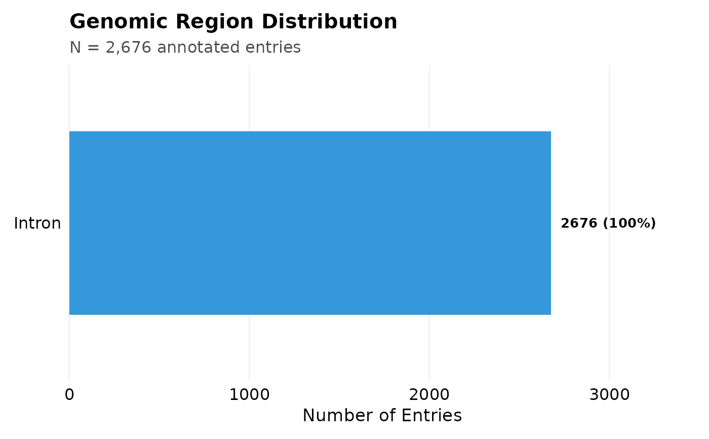
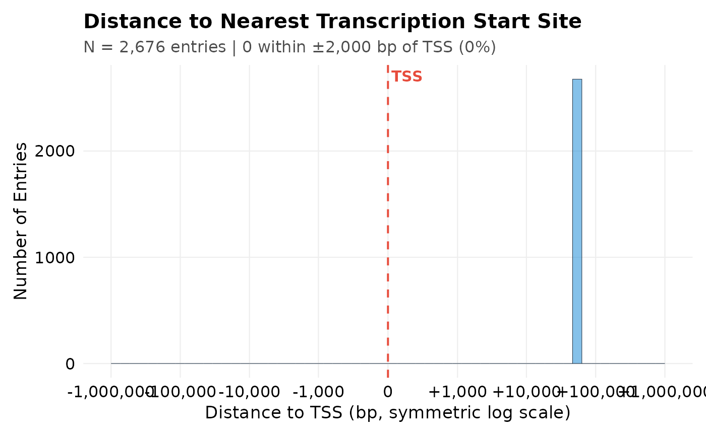
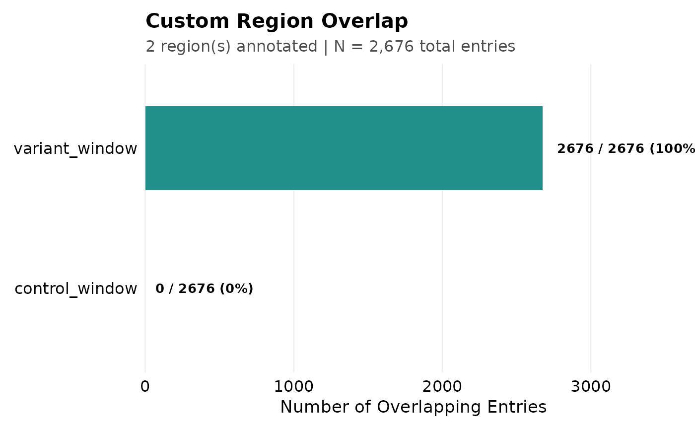
"region": Bar chart ofregion_typedistribution (hierarchical: cds, 5utr, 3utr, intron, promoter, intergenic)."tss": Density plot ofdist_to_tsson a symmetric log10 scale, showing how far variants are from the nearest TSS."custom": Bar chart counting variants overlapping with user-defined custom regions (booleanis_*/in_*columns created byav_annotate_regions).
Usage
av_plot_annotation(
  obj,
  type = c("region", "tss", "custom"),
  proximal_window = 2000
)
Arguments
- obj
An object of class
AlphaVarSet. Must contain annotation columns produced byav_annotate_genes()and/orav_annotate_regions().- type
Character. One of
"region","tss", or"custom".- proximal_window
Integer (bp). For
type = "tss"only: half-width of the window around the TSS used to compute the "proximal" fraction shown in the subtitle. Default2000matches the promoter definition used byav_annotate_genes().
Interpretation
The distribution reflects the genomic context of scored variants. A high proportion of intronic/intergenic variants is typical for regulatory scores. Enrichment in CDS or UTR regions compared to genomic background may indicate protein-coding or post-transcriptional regulatory effects. Compare to the expected genome-wide distribution (~1-2% CDS, ~25% intronic, ~45% intergenic) to identify deviations.
Examples
example_file <- system.file("extdata", "bcl11a_rs1427407_example.csv",
package = "AlphaVaR")
obj <- av_import_csv(example_file)
#> Reading bcl11a_rs1427407_example.csv ...
# type = "custom" needs no TxDb: av_annotate_regions() accepts any GRanges.
windows <- GenomicRanges::GRanges(
seqnames = "chr2",
ranges = IRanges::IRanges(
start = c(60489908, 60590000),
end = c(60491908, 60592000)
)
)
obj <- av_annotate_regions(obj, windows[1], label = "is_variant_window")
obj <- av_annotate_regions(obj, windows[2], label = "is_control_window")
obj$meta$custom_regions
#> [1] "is_variant_window" "is_control_window"
av_plot_annotation(obj, type = "custom")
 # "region" and "tss" read the columns av_annotate_genes() adds, so they need
# the hg38 TxDb, a ~1 GB Suggests package.
if (requireNamespace("TxDb.Hsapiens.UCSC.hg38.knownGene", quietly = TRUE)) {
obj <- av_annotate_genes(obj)
print(table(obj$data$region_type))
print(av_plot_annotation(obj, type = "region"))
print(av_plot_annotation(obj, type = "tss", proximal_window = 2000))
}
#> Extracting gene information from annotation database...
#> Calculating strand-aware distances to nearest TSS...
#> Resolving gene symbols...
#> 'select()' returned 1:1 mapping between keys and columns
#> Classifying genomic regions (hierarchical)...
#> Annotation complete.
#>
#> intron
#> 2676
# "region" and "tss" read the columns av_annotate_genes() adds, so they need
# the hg38 TxDb, a ~1 GB Suggests package.
if (requireNamespace("TxDb.Hsapiens.UCSC.hg38.knownGene", quietly = TRUE)) {
obj <- av_annotate_genes(obj)
print(table(obj$data$region_type))
print(av_plot_annotation(obj, type = "region"))
print(av_plot_annotation(obj, type = "tss", proximal_window = 2000))
}
#> Extracting gene information from annotation database...
#> Calculating strand-aware distances to nearest TSS...
#> Resolving gene symbols...
#> 'select()' returned 1:1 mapping between keys and columns
#> Classifying genomic regions (hierarchical)...
#> Annotation complete.
#>
#> intron
#> 2676