AlphaVaR: Statistical Interpretation of AlphaGenome Variant-Effect Predictions

Warnings and messages are left visible throughout. Several of them report a decision the analysis made on your behalf, such as a dropped low-coverage group or a column that carries structural NAs. They are part of what the output means.

Introduction

One variant, thousands of tracks

AlphaGenome reads up to one megabase of DNA and predicts functional genomic tracks across eleven modalities, among them chromatin accessibility, histone marks, transcription-factor binding, transcription and splicing, at single-base resolution. For every track it returns two numbers: a raw score for the physical magnitude of the predicted change, and a quantile score giving the percentile rank of that magnitude within a genome-wide background of common variants.

A single queried variant therefore yields thousands of scored tracks, each annotated by modality, tissue, assay and finer descriptors, and returned in a long variant scoring CSV. Identifying which of those tracks carry signal above the background is the step AlphaVaR provides.

What AlphaVaR adds

A typed object that holds the full variant scoring CSV together with every result computed on it and a record of how the data was filtered.
Localization tests that ask where extreme scores or shifted distributions concentrate, with Benjamini-Hochberg correction and an effect size beside every p-value.
A specificity index ( $\tau$ ) measuring how far an effect concentrates on a few elements of a chosen variable.
A transparent prioritization that ranks candidates across interpretable criteria and maps each to a target gene, without collapsing the criteria into one synthetic score.
Plots, reproducible reports and a code-free Shiny application over all of the above.

AlphaVaR performs variant-level epigenomic interpretation and conditional prioritization within a locus. It does not infer phenotype-level causality: which tissue mediates a trait, or which mechanism drives it, needs external evidence such as GWAS-tissue colocalization or eQTL fine-mapping.

The one engine

The tests and metrics are parameterized by two variables rather than specialized per question: per, the variable that defines the unit summarized, and across, the variable being analyzed. The same tests run unchanged on any column, so the choice of column sets the question. Modality, tissue, transcription factor and gene are all answered by the same machinery.

The example data

Every chunk below runs on the complete AlphaGenome output for rs1427407, which ships with the package gzipped as inst/extdata/bcl11a_rs1427407_scores.csv.gz: 71,420 scored rows over the two alternate alleles, 11 modalities, 715 biosamples and 751 profiled transcription factors, in the full 25-column schema. Nothing here needs network access, and the numbers printed below are the ones reported for this variant.

A seeded stratified subset of the same table, bcl11a_rs1427407_example.csv, ships alongside it and backs the help-page examples and the test suite, where a small file keeps runtimes short. It caps each modality at a fixed number of rows, which makes it good for exercising the schema and unsuitable for the enrichment tests, whose results depend on the relative sizes of the modalities.

Quick start

library(AlphaVaR)

# One call: import, compute statistics, launch the interactive app.
# Not evaluated here because it starts a Shiny server and blocks the session.
av_explore(system.file("extdata", "bcl11a_rs1427407_scores.csv.gz", package = "AlphaVaR"))

The typed object

av_import_csv() keeps every original column, preserves the canonical AlphaGenome names and compresses repeated metadata to factors, so an output with tens of thousands of tracks stays compact in memory.

CSV column	Required?	Description
`variant_id`	Yes	Variant identifier (`chr:pos:ref>alt`)
`quantile_score` / `raw_score`	One required	Rarity against the common-variant background / physical magnitude. `quantile_score` is the active score on import
`output_type`	No	Modality
`biosample_name`	No	Tissue or cell type
`gene_name`	No	Gene annotated to the track
`scored_interval`	No	Genomic coordinates

Only variant_id and at least one score column are required. Every other column is preserved and can be used as per or across.

library(AlphaVaR)

obj <- av_import_csv(
  file = system.file("extdata", "bcl11a_rs1427407_scores.csv.gz", package = "AlphaVaR")
)
#> Reading bcl11a_rs1427407_scores.csv.gz ...

obj
#> === AlphaVarSet Object ===
#> Entries:    71,420 
#> Variants:   2 
#> Modalities: 11 
#> Columns:    25 (incl. 19 extra)
#> Score Mode: quantile_score 
#> Source:     bcl11a_rs1427407_scores.csv.gz

A single AlphaVarSet can hold more than one variant, including the distinct alternate alleles at one position, each keyed by its variant_id. AlphaGenome scores one alternate allele per run, so the T>C and T>G alleles of rs1427407 are imported into one object and analyzed together as an allelic series.

av_overview_summary(obj)
#> === AlphaVarOverview Summary ===
#> Score: quantile_score | mean: 0.2692  median: 0.2751  (unbalanced)
#> 
#> # A tibble: 8 × 7
#>   field              n_unique pct_unique n_missing pct_missing n_empty pct_empty
#>   <chr>                 <int>      <dbl>     <int>       <dbl>   <int>     <dbl>
#> 1 entries               71420     100            0        0          0         0
#> 2 variant_id                2       0            0        0          0         0
#> 3 scored_interval           1       0            0        0          0         0
#> 4 gene_name                23       0.03     15108       21.2        0         0
#> 5 output_type              11       0.02         0        0          0         0
#> 6 transcription_fac…      751       1.05     64952       90.9        0         0
#> 7 histone_mark             29       0.04     66956       93.8        0         0
#> 8 biosample_name          714       1            4        0.01       0         0

Switching the active score

The active score, physical effect or rarity, is switched with av_set_active_score(). Any cached result is discarded whenever the rows or the active score change, so a statistic can never be read against the wrong data. The switch reports what it did:

raw_obj <- av_set_active_score(obj, "raw")   # "quantile" or "raw", not the column name
#> Switched active score: quantile_score -> raw_score. Statistics cleared.
raw_obj$meta$active_score
#> [1] "raw_score"

Once statistics have been computed, the same call empties them; the section on localization tests below shows that.

The rest of this vignette stays on the quantile score. That is the domain the rarity threshold is defined on, and the one in which tissue specificity is interpretable. $\tau$ itself can be computed on either score.

Which modalities carry the effect?

Asking whether a modality stands out covers two distinct questions, and AlphaVaR answers them with two distinct functions.

av_calc_enrichment() runs a one-vs-rest Fisher’s exact test: are extreme scores over-represented in this group? “Extreme” means at or above the rarity threshold in absolute value, so strongly negative quantile scores count as well. The threshold defaults to the top 5 % of the quantile score.

obj <- av_calc_enrichment(obj, group_by = "output_type")
#> av_calc_enrichment: using default hit threshold 0.95 (top-5% quantile_score rarity).
#> This message is displayed once per session.

obj$stats$comparisons[["enrichment"]]$fisher_tidy
#> # A tibble: 11 × 8
#>    group           n_obs n_hits      or log2OR     p_raw     p_adj neg_log10_fdr
#>    <fct>           <int>  <int>   <dbl>  <dbl>     <dbl>     <dbl>         <dbl>
#>  1 SPLICE_JUNCTIO… 18350      3 8.89e-3 -6.82  7.47e-119 8.21e-118       117.   
#>  2 CAGE             2184    206 9.42e+0  3.24  1.33e-110 7.32e-110       109.   
#>  3 ATAC              668    119 1.80e+1  4.17  7.95e- 95 2.91e- 94        93.5  
#>  4 CHIP_HISTONE     4464    195 3.94e+0  1.98  1.17e- 48 3.21e- 48        47.5  
#>  5 RNA_SEQ         37224    348 5.15e-1 -0.957 1.24e- 23 2.73e- 23        22.6  
#>  6 CHIP_TF          6468     59 6.52e-1 -0.617 1.01e-  3 1.86e-  3         2.73 
#>  7 DNASE            1220     26 1.61e+0  0.687 2.33e-  2 3.66e-  2         1.44 
#>  8 SPLICE_SITE_US…   734      7 7.02e-1 -0.510 4.23e-  1 5.81e-  1         0.235
#>  9 SPLICE_SITES        4      0 0        3.02  1   e+  0 1   e+  0         0    
#> 10 CONTACT_MAPS       56      0 0       -0.629 1   e+  0 1   e+  0         0    
#> 11 PROCAP             48      0 0       -0.409 1   e+  0 1   e+  0         0

n_obs counts scored rows, not unique genomic variants. One row is one variant scored on one track, and a track can appear more than once for the same variant where several variant scorers or gene annotations apply. This file holds 71,420 rows over 2 variants and 4,619 track names. Keeping the unit straight matters for every count in this vignette.

av_calc_shift() runs rank-based shift tests: does this group’s whole score distribution sit above or below the background? It sweeps every element of the column with a Wilcoxon-Mann-Whitney test and adds a Kruskal-Wallis omnibus.

obj <- av_calc_shift(obj, group_by = "output_type")
#> Warning: 1 element(s) dropped (n < 5 in one arm): SPLICE_SITES

obj$stats$comparisons[["output_type_vs_rest"]]$results_tidy
#> # A tibble: 10 × 12
#>    group n_group n_rest median_group median_rest median_diff     p_val     p_adj
#>    <chr>   <int>  <int>        <dbl>       <dbl>       <dbl>     <dbl>     <dbl>
#>  1 ATAC      668  70752        0.818       0.344     0.474   0         0        
#>  2 CAGE     2184  69236        0.705       0.339     0.367   0         0        
#>  3 CHIP…    4464  66956        0.630       0.333     0.297   0         0        
#>  4 DNASE    1220  70200        0.517       0.344     0.173   0         0        
#>  5 CHIP…    6468  64952        0.460       0.334     0.126   0         0        
#>  6 SPLI…   18350  53070        0.284       0.392    -0.108   0         0        
#>  7 RNA_…   37224  34196        0.312       0.376    -0.0635  1.19e-100 1.70e-100
#>  8 CONT…      56  71364        0.535       0.344     0.191   2.55e-  5 3.19e-  5
#>  9 PROC…      48  71372        0.565       0.344     0.221   1.66e-  3 1.85e-  3
#> 10 SPLI…     734  70686        0.349       0.344     0.00522 4.48e-  1 4.48e-  1
#> # ℹ 4 more variables: effect_size <dbl>, effect_type <chr>, method <chr>,
#> #   significance_stars <chr>

Both are Benjamini-Hochberg corrected and both report an effect size beside the p-value: a log odds ratio for Fisher, a rank-biserial $r$ and a median difference for the shift test. Pooling thousands of rows lets trivially small effects reach significance, so the effect size carries the interpretation. Read the direction off median_diff and the magnitude off abs(effect_size).

The two tests do not have to agree, and where they disagree the disagreement is the result. CONTACT_MAPS has not a single row in the top 5 %, so Fisher has nothing to weigh and returns p_adj 1.00, while its distribution as a whole sits clearly above the background (median difference +0.19, shift p_adj 3.2e-05). A distribution can move without any single row reaching the tail, and a threshold test cannot see that. PROCAP behaves the same way.

The two functions also differ in their power guard. The shift sweep carries min_n = 5 and drops SPLICE_SITES, which has four rows here. av_calc_enrichment() has no such guard and reports it. The guard removes small-sample artefacts, but it can also drop a genuine low-coverage group, so descriptive ranking suits discovery and the tests suit well-covered groups.

av_calc_shift() sweeps every element of the column. To test one element on its own, av_compare_target() takes the column and the value and writes the key <column>=<value>, or <column>_vs_rest for a logical column.

Each result lives under its own key in $stats$comparisons, so they coexist:

names(obj$stats$comparisons)
#> [1] "enrichment"          "output_type_vs_rest"

Now that results are cached, the invalidation contract becomes visible: changing the active score discards them, because they were computed against the other score.

length(av_set_active_score(obj, "raw")$stats)
#> Switched active score: quantile_score -> raw_score. Statistics cleared.
#> [1] 0

Correcting for track imbalance

The tests above treat every row as an independent observation, and where both alleles were scored on the same track that track is counted twice. balance_by collapses each arm to one value per unit before testing:

balanced <- av_calc_shift(
  obj,
  group_by   = "output_type",
  balance_by = "variant_id",
  per        = "track_name"
)
#> Warning: 1 element(s) dropped (n < 5 in one arm): SPLICE_SITES

balanced$stats$comparisons[["output_type_vs_rest"]]$results_tidy[, c(
  "group", "n_group", "median_diff", "effect_size", "p_adj", "significance_stars"
)]
#> # A tibble: 10 × 6
#>    group            n_group median_diff effect_size     p_adj significance_stars
#>    <chr>              <int>       <dbl>       <dbl>     <dbl> <chr>             
#>  1 ATAC                 167     0.270       -0.699  0         ***               
#>  2 CAGE                 273     0.197       -0.549  0         ***               
#>  3 CHIP_HISTONE        1116     0.155       -0.378  0         ***               
#>  4 SPLICE_JUNCTIONS     367    -0.206        0.748  5.01e-125 ***               
#>  5 RNA_SEQ              371    -0.131        0.405  4.54e- 38 ***               
#>  6 SPLICE_SITE_USA…     367    -0.114        0.356  1.33e- 29 ***               
#>  7 CHIP_TF             1617    -0.00965      0.0749 3.74e-  5 ***               
#>  8 DNASE                305     0.00890     -0.0496 1.84e-  1 ns                
#>  9 CONTACT_MAPS          28     0.0284      -0.103  3.87e-  1 ns                
#> 10 PROCAP                 6     0.0339      -0.0911 6.99e-  1 ns

Every one of the 4,619 track names is scored for both alleles here, so the collapse removes that duplication completely, and it also averages over the repeated rows within one variant and track. The group sizes fall accordingly.

One call flips: DNase is a strong upward shift on the raw rows and drops to ns once the arms are collapsed. Its unbalanced signal came from repeated measurements of the same tracks rather than from independent evidence, which is exactly the pseudo-replication balance_by exists to remove. Read the balanced table when the question is whether an effect is real, and the unbalanced one only to see how much of it rests on coverage.

Two constraints on the arguments. group_by, balance_by and per must be three different columns, so balancing by variant_id here requires an explicit per. And per has to name a genuinely replicated unit: with the documented default per = "variant_id" this two-allele file offers two units, which is below min_n for every element.

Two views of the result

av_plot_enrichment(obj, style = "volcano", label_top_n = 5)
#> Fewer than 15 enrichment groups. Consider style = "bar" for small group counts.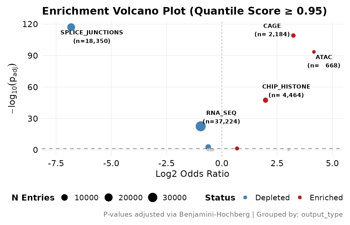

Fisher enrichment: log2 odds ratio against -log10 FDR. Points are sized by the number of scored rows in the group.

av_plot_comparison(obj, comparison_name = "output_type_vs_rest")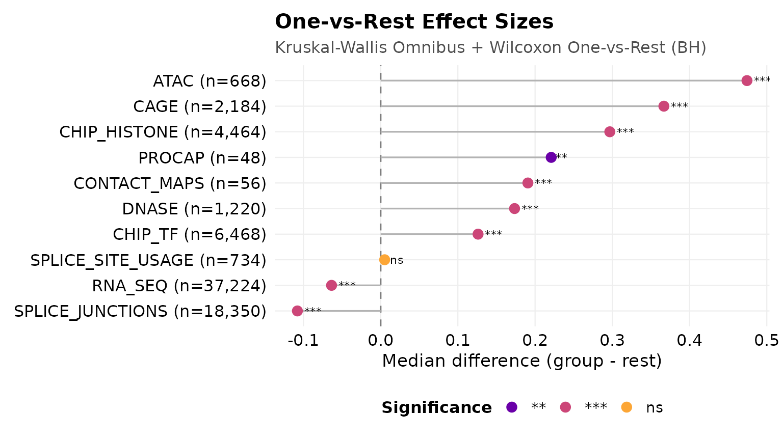

One-vs-rest shift test per modality. The comparison_name argument is passed explicitly, or the first stored comparison is rendered instead.

av_plot_distribution(obj, style = "ridges")
#> Picking joint bandwidth of 0.061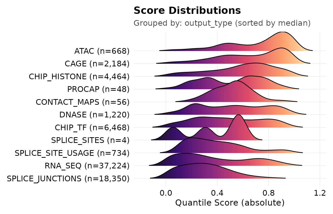

Score distributions per modality, sorted by median absolute score.

av_plot_distribution(obj, style = "directionality")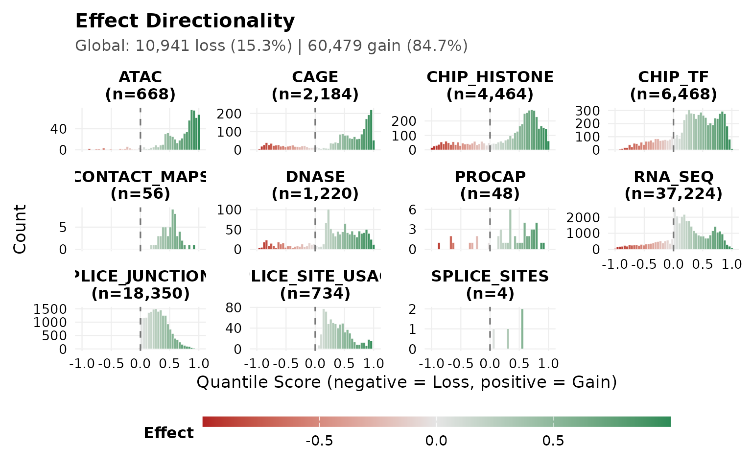

Balance between negative and positive quantile-score effects, per modality.

In which tissue or cell type does it act?

$\tau$ , the specificity index of Yanai et al. (2005), measures how far an effect concentrates on a few elements of a chosen variable. It is bounded on $[0, 1]$ and comparable across columns of different size: $\tau \rightarrow 0$ is a uniform effect, $\tau \rightarrow 1$ an effect concentrated on a single element. It is descriptive and carries no p-value.

Read across all biosamples at once, both alleles look broad:

obj <- av_calc_specificity(obj, across = "biosample_name", metric = "both")
#> Warning: av_calc_specificity: dropped 4/71420 rows with NA in quantile_score,
#> biosample_name, or variant_id.

obj$stats$specificity[["biosample_name"]]
#> # A tibble: 2 × 5
#>   variant_id        specificity n_active n_elements top_element
#>   <chr>                   <dbl>    <int>      <int> <chr>      
#> 1 chr2:60490908:T>C       0.102      348        714 heart      
#> 2 chr2:60490908:T>G       0.136      138        714 K562

That is dilution, not an answer. Pooling mixes channels whose scores sit at different levels, so a pooled $\tau$ is not a statement about any one of them. A variant can look broad pooled over all modalities and still be tissue-specific within the modality that reports the element’s activity. Reading tissue specificity per modality separates the channels:

obj <- av_calc_specificity(
  obj,
  per     = "output_type",
  across  = "biosample_name",
  metric  = "both"
)
#> Warning: av_calc_specificity: dropped 4/71420 rows with NA in quantile_score,
#> biosample_name, or output_type.

obj$stats$specificity[["biosample_name"]]
#> # A tibble: 10 × 5
#>    output_type       specificity n_active n_elements top_element                
#>    <fct>                   <dbl>    <int>      <int> <chr>                      
#>  1 ATAC                   0.0620      118        167 naive B cell               
#>  2 CAGE                   0.0858       73        264 bone marrow cell           
#>  3 CHIP_HISTONE           0.153        52        219 CD14-positive monocyte     
#>  4 CHIP_TF                0.258        11        163 HL-60                      
#>  5 CONTACT_MAPS           0.311         0         12 GM12878                    
#>  6 DNASE                  0.295        23        305 hematopoietic multipotent …
#>  7 PROCAP                 0.188         0          6 K562                       
#>  8 RNA_SEQ                0.0559      151        285 heart                      
#>  9 SPLICE_JUNCTIONS       0.267         2        282 K562                       
#> 10 SPLICE_SITE_USAGE      0.401         7        282 thoracic aorta

SPLICE_SITES is absent because its four rows are the only ones without a biosample_name, and the warning above says so.

$\tau$ has to be read together with n_active, the number of elements that reach the rarity threshold. CONTACT_MAPS and PROCAP carry a mid-range $\tau$ on n_active of zero: $\tau$ measures how concentrated a profile is, not how strong it is, so a channel in which the variant does nothing scores on a concentrated noise profile. A low $\tau$ over many active elements says the response is broad; a $\tau$ over none says nothing at all. Across the four channels the enrichment table marked as enriched, $\tau$ runs from 0.06 in ATAC, the most strongly enriched and the broadest, to 0.30 in DNase, the weakest of the four and the most concentrated. Strength and specificity are separate readings.

The slot is keyed by across, not by per, so the second call replaced the first under biosample_name. Two specificity results over the same across variable cannot be held at once; keep the one you need, or recompute.

av_plot_specificity(obj, style = "tau", across = "biosample_name")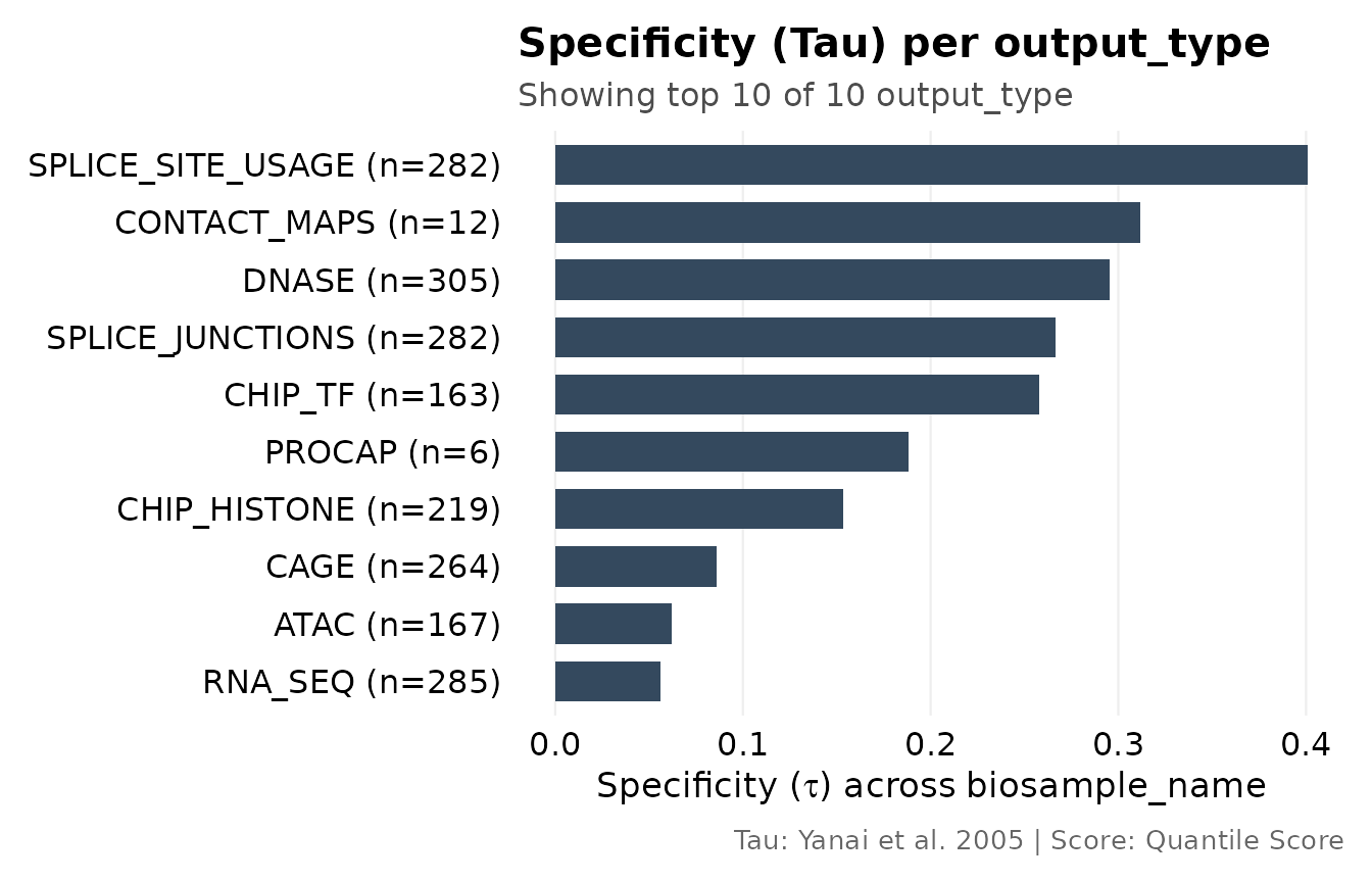

Tissue specificity per modality. The tau style is requested explicitly, because the default style needs a prioritization result.

Specificity is a property of the channel it is read in, not of the variant alone, and conditioning on one channel shows that. DNase is the channel of interest here for a reason external to the data, namely that rs1427407 marks a DNase-hypersensitive site. Subsetting resets $stats, so $\tau$ is computed after the filter:

dnase <- av_subset(obj, output_type == "DNASE", .description = "DNase rows")
dnase <- av_calc_specificity(dnase, across = "biosample_name", metric = "both")

dnase$stats$specificity[["biosample_name"]]
#> # A tibble: 2 × 5
#>   variant_id        specificity n_active n_elements top_element                 
#>   <chr>                   <dbl>    <int>      <int> <chr>                       
#> 1 chr2:60490908:T>C       0.329       22        305 hematopoietic multipotent p…
#> 2 chr2:60490908:T>G       0.374        2        305 immature natural killer cell

Inside DNase, per-allele $\tau$ is roughly three times the pooled value, and the leading biosample for T>C is a hematopoietic multipotent progenitor. Read n_active alongside it: T>C has 22 active biosamples against T>G’s two, so the T>C row is the one that carries an interpretable signal.

Conditioning does not raise $\tau$ everywhere, and that is the point rather than a caveat. Inside ATAC, the most strongly enriched channel of all, $\tau$ for T>C is lower than the pooled value: the variant moves ATAC signal in many biosamples at once, which is breadth, not specificity. Specificity and enrichment answer different questions, and which channel to condition on is decided by the localization tests and by what the assay measures, not by $\tau$ .

One table instead of three calls

av_element_summary() assembles the descriptive summary, the Fisher block, the shift block and $\tau$ for one column in a single read-only call. It returns a plain tibble and writes nothing to $stats.

mods <- av_element_summary(
  obj,
  element            = "output_type",
  tests              = c("enrichment", "shift", "specificity"),
  specificity_across = "biosample_name"
)
#> Warning: 1 element(s) dropped (n < 5 in one arm): SPLICE_SITES
#> Warning: av_calc_specificity: dropped 4/71420 rows with NA in quantile_score,
#> biosample_name, or output_type.

mods[, c("output_type", "n_tracks", "fisher_log2OR", "fisher_q",
         "wilcox_median_diff", "wilcox_q")]
#> # A tibble: 11 × 6
#>    output_type    n_tracks fisher_log2OR  fisher_q wilcox_median_diff   wilcox_q
#>    <chr>             <int>         <dbl>     <dbl>              <dbl>      <dbl>
#>  1 RNA_SEQ           37224        -0.957 2.73e- 23           -0.0635   1.70e-100
#>  2 CHIP_HISTONE       4464         1.98  3.21e- 48            0.297    0        
#>  3 DNASE              1220         0.687 3.66e-  2            0.173    0        
#>  4 CHIP_TF            6468        -0.617 1.86e-  3            0.126    0        
#>  5 CAGE               2184         3.24  7.32e-110            0.367    0        
#>  6 ATAC                668         4.17  2.91e- 94            0.474    0        
#>  7 SPLICE_SITE_U…      734        -0.510 5.81e-  1            0.00522  4.48e-  1
#>  8 SPLICE_JUNCTI…    18350        -6.82  8.21e-118           -0.108    0        
#>  9 PROCAP               48        -0.409 1   e+  0            0.221    1.85e-  3
#> 10 CONTACT_MAPS         56        -0.629 1   e+  0            0.191    3.19e-  5
#> 11 SPLICE_SITES          4         3.02  1   e+  0           NA       NA    

mods[, c("output_type", "spec_tau", "spec_n_active", "spec_top_element")]
#> # A tibble: 11 × 4
#>    output_type       spec_tau spec_n_active spec_top_element                    
#>    <chr>                <dbl>         <int> <chr>                               
#>  1 RNA_SEQ             0.0559           151 heart                               
#>  2 CHIP_HISTONE        0.153             52 CD14-positive monocyte              
#>  3 DNASE               0.295             23 hematopoietic multipotent progenito…
#>  4 CHIP_TF             0.258             11 HL-60                               
#>  5 CAGE                0.0858            73 bone marrow cell                    
#>  6 ATAC                0.0620           118 naive B cell                        
#>  7 SPLICE_SITE_USAGE   0.401              7 thoracic aorta                      
#>  8 SPLICE_JUNCTIONS    0.267              2 K562                                
#>  9 PROCAP              0.188              0 K562                                
#> 10 CONTACT_MAPS        0.311              0 GM12878                             
#> 11 SPLICE_SITES       NA                 NA NA

fisher_sig in the full table is effect-size gated and is therefore TRUE for depletion as well as enrichment; read the sign of fisher_log2OR with it.

A column that is populated only inside part of the data is a nested sub-parameter rather than a full-rank column: transcription_factor exists inside CHIP_TF and histone_mark inside CHIP_HISTONE, while gene_name is filled in the four gene-resolved modalities. Using such a column as element without first subsetting to its parent modalities mixes structural NAs and drops most of the data. Subset first:

tf <- av_subset(obj, output_type == "CHIP_TF", .description = "TF-binding tracks")

tf_ranking <- av_element_summary(tf, element = "transcription_factor",
                                 tests = character(0))
head(tf_ranking[, c("transcription_factor", "max_abs_score", "n_tracks")], 10)
#> # A tibble: 10 × 3
#>    transcription_factor max_abs_score n_tracks
#>    <chr>                        <dbl>    <int>
#>  1 SPI1                         0.997       16
#>  2 ZNF384                       0.994       16
#>  3 TEAD4                        0.985       32
#>  4 GATA2                        0.980       24
#>  5 POLR2AphosphoS5              0.980      104
#>  6 TCF3                         0.979        8
#>  7 SMARCE1                      0.974        8
#>  8 TAL1                         0.974        4
#>  9 ATF1                         0.972       16
#> 10 ARID1B                       0.971        4

This is where a coverage filter would do damage. TAL1 reaches the top ten on four scored rows, and so do the other members of the erythroid master-regulator complex:

tf_ranking[tf_ranking$transcription_factor %in%
             c("TAL1", "GATA1", "CBFA2T3", "CBFA2T2"),
           c("transcription_factor", "max_abs_score", "n_tracks")]
#> # A tibble: 4 × 3
#>   transcription_factor max_abs_score n_tracks
#>   <chr>                        <dbl>    <int>
#> 1 TAL1                         0.974        4
#> 2 GATA1                        0.970        4
#> 3 CBFA2T3                      0.955        4
#> 4 CBFA2T2                      0.936        4

Four rows here means one K562 track counted for both alleles and both variant scorers, which is what n_tracks reports: rows, as everywhere else. A min_n = 5 guard would drop all four factors and leave broadly profiled ones such as ZNF384, at 16 rows, at the top. That is why no test was requested here. The ranking is descriptive and coverage is printed beside it, so the reader can see what each position rests on.

Which gene is the target?

av_map_targets() assigns each variant a target gene in two tiers. Tier 1 (Direct) names the highest-scoring gene among the gene-annotated tracks that pass the rarity threshold, so the call follows the predicted functional signal, and the full qualifying set is kept in all_target_genes. Tier 2 (Distal) is a labelled fallback for variants with no gene-annotated track above the threshold: it reports the nearest gene and marks the variant as lacking direct evidence.

distance_to_tss needs the annotation step, which is why it runs first:

# TxDb and org.Hs.eg.db are Suggests; where they are installed this runs for
# real, and elsewhere it is skipped rather than faked. suppressMessages() hides
# the TxDb boilerplate along with av_annotate_genes()' own progress messages.
if (requireNamespace("TxDb.Hsapiens.UCSC.hg38.knownGene", quietly = TRUE) &&
    requireNamespace("org.Hs.eg.db", quietly = TRUE)) {
  obj <- suppressMessages(
    av_annotate_genes(obj, txdb_package = "TxDb.Hsapiens.UCSC.hg38.knownGene")
  )
  print(table(obj$data$region_type, useNA = "ifany"))
}
#> 
#> 
#> intron 
#>  71420

obj <- av_map_targets(obj)

obj$stats$targets[["variant_id"]][, c(
  "variant_id", "target_gene", "evidence_tier", "n_target_genes", "distance_to_tss"
)]
#> # A tibble: 2 × 5
#>   variant_id        target_gene     evidence_tier n_target_genes distance_to_tss
#>   <chr>             <chr>           <chr>                  <int>           <dbl>
#> 1 chr2:60490908:T>C BCL11A          Tier 1 (Dire…              6           51066
#> 2 chr2:60490908:T>G ENSG00000233953 Tier 1 (Dire…              7           51066

Both alleles reach Tier 1 here, and they name different genes: the tier records whether a gene-annotated row cleared the rarity threshold, and the gene is the highest-scoring one among those that did. n_target_genes shows how many genes qualified, all_target_genes lists them, and supporting_tfs and supporting_marks hold the evidence behind the call. A single top gene is a starting point for follow-up, not a verdict, which is why the qualifying set is kept.

Two properties of distance_to_tss matter when reading the table. It is the distance to the nearest gene at that coordinate, which is gene_symbol in obj$data, with nearest_gene beside it holding the Entrez ID. For a Tier-2 row the two coincide, because Tier 2 is the nearest gene; for a Tier-1 row the distance does not describe target_gene. Both columns exist only once av_annotate_genes() has run, and distance_to_tss is NA until then. The distance is recorded as information only. It never weights the ranking.

Which candidate leads?

av_prioritize() ranks variants on $K$ independently interpretable criteria (three by default), with no learned or hand-set weighting: the strongest absolute per-track effect (magnitude), the tissue specificity $\tau$ , and the number of tracks reaching the rarity threshold (evidence breadth). Each criterion is mapped to its within-cohort percentile rank $r_k \in [0, 1]$ and the summary rank is their mean,

$\mathrm{priority\ rank}_v = \frac{1}{K}\sum_{k=1}^{K} r_k(v)$

reported alongside the Pareto front: the set of variants that no other variant equals or beats on every criterion while beating it on at least one. A variant that leads on one criterion but falls mid-field on the others has a moderate mean rank and still lies on the front, so the two quantities are read together. The priority rank orders candidates within a locus and carries no significance interpretation.

Percentile ranks are within-cohort quantities and need a cohort. The example data ships two alleles of a single variant, where percent_rank() can only return 0 or 1, and neither allele dominates the other, so the front holds both and separates nothing. The calls are therefore shown rather than run:

obj <- av_prioritize(obj)
obj$stats$prioritization[["variant_id"]]

av_plot_priority(obj)

On a real multi-variant cohort, such as the candidates in a fine-mapped credible set, both the mean rank and the front are informative.

Working the object

Filters are chainable, reset $stats, and are recorded.

high_rarity <- av_subset(obj, abs(quantile_score) >= 0.95,
                         .description = "top-5% rarity")
high_rarity
#> === AlphaVarSet Object ===
#> Entries:    963 
#> Variants:   2 
#> Modalities: 8 
#> Columns:    29 (incl. 23 extra)
#> Score Mode: quantile_score 
#> Source:     bcl11a_rs1427407_scores.csv.gz

top_rows <- av_get_top(obj, n = 20)
nrow(top_rows$data)
#> [1] 20

By default av_get_top() selects scored rows, not variants: n = 20 returns twenty rows, which on this file belong to the same two variants. Pass group_by = "variant_id" to make n count whole groups instead.

filtered <- obj |>
  av_subset(output_type == "CHIP_HISTONE", .description = "Histone ChIP tracks") |>
  av_get_top(n = 50)

av_print_breadcrumbs(filtered)
#> All Data (71,420) -> Histone ChIP tracks (4,464) -> Top 50 entries by quantile_score (50)

Comparing the two alleles

av_compare_groups() stratifies: it compares the groups of group_by within each item of compare_by. Here the two alternate alleles are the groups and each modality is an item, so the T>C-versus-T>G contrast is tested modality by modality.

obj <- av_compare_groups(obj, group_by = "variant_id", compare_by = "output_type")
#> Warning: 1 items skipped due to insufficient sample size (n < 5 ): SPLICE_SITES

head(obj$stats$comparisons[["variant_id_by_output_type"]]$results_tidy)
#> # A tibble: 6 × 16
#>   item        group_1 group_2   n_1   n_2 median_1 median_2 median_diff    p_val
#>   <chr>       <chr>   <chr>   <int> <int>    <dbl>    <dbl>       <dbl>    <dbl>
#> 1 SPLICE_SIT… chr2:6… chr2:6…   367   367    0.494    0.257      0.237  0       
#> 2 ATAC        chr2:6… chr2:6…   334   334    0.896    0.708      0.188  0       
#> 3 CAGE        chr2:6… chr2:6…  1092  1092    0.784    0.642      0.143  0       
#> 4 SPLICE_JUN… chr2:6… chr2:6… 10643  7707    0.270    0.308     -0.0379 3.34e-37
#> 5 CHIP_TF     chr2:6… chr2:6…  3234  3234    0.487    0.441      0.0466 5.61e-11
#> 6 CHIP_HISTO… chr2:6… chr2:6…  2232  2232    0.649    0.614      0.0347 2.99e- 7
#> # ℹ 7 more variables: effect_size <dbl>, effect_type <chr>, method <chr>,
#> #   epsilon_sq <dbl>, kw_p <dbl>, p_adj <dbl>, significance_stars <chr>

av_plot_comparison(obj, comparison_name = "variant_id_by_output_type")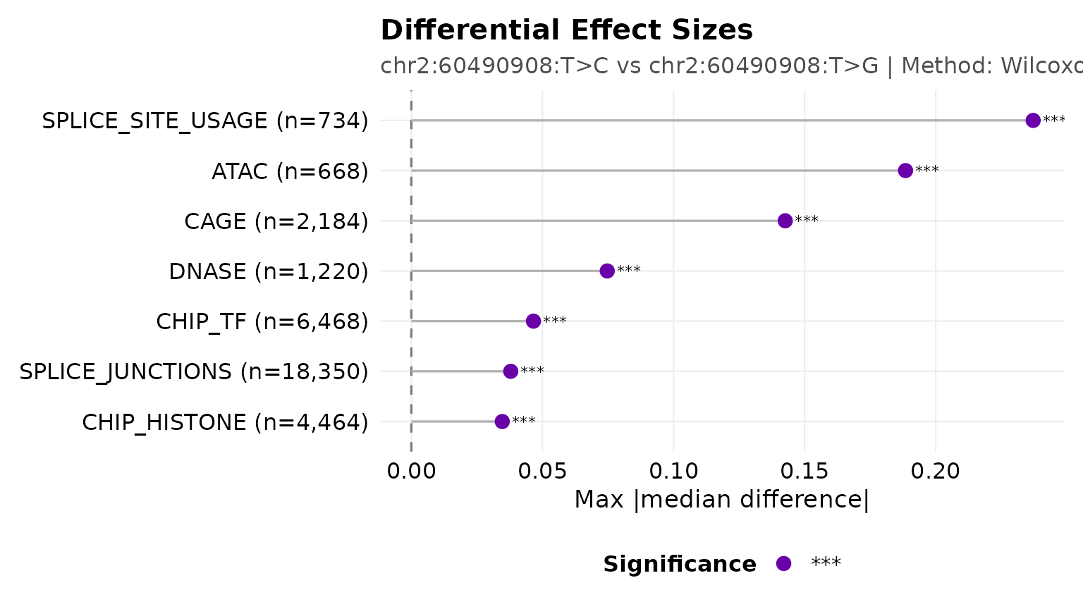

Allele contrast: each modality tested for a T>C versus T>G difference.

Two-group comparisons and many-to-one reference comparisons have no valid omnibus, so global_p is NA_real_ for them by convention rather than the minimum of the pairwise p-values, which would be an implicit selection step.

Genomic context

av_plot_interval() draws the scored interval AlphaGenome was run over, with every variant in the object placed on it:

av_plot_interval(obj)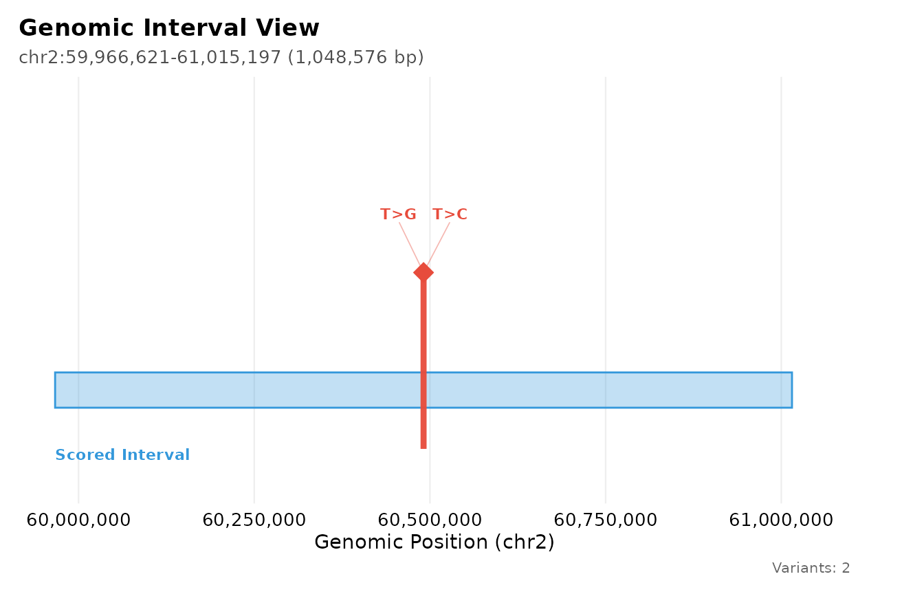

The 1 Mb scored interval, with both alternate alleles of rs1427407 marked at their shared coordinate.

av_plot_locus() zooms to one gene and splits the scores by modality. It needs several variants spread over the locus to be informative; here both alleles sit on the same base, so each modality panel collapses to a single vertical stack:

av_plot_locus(obj, gene_name = "BCL11A")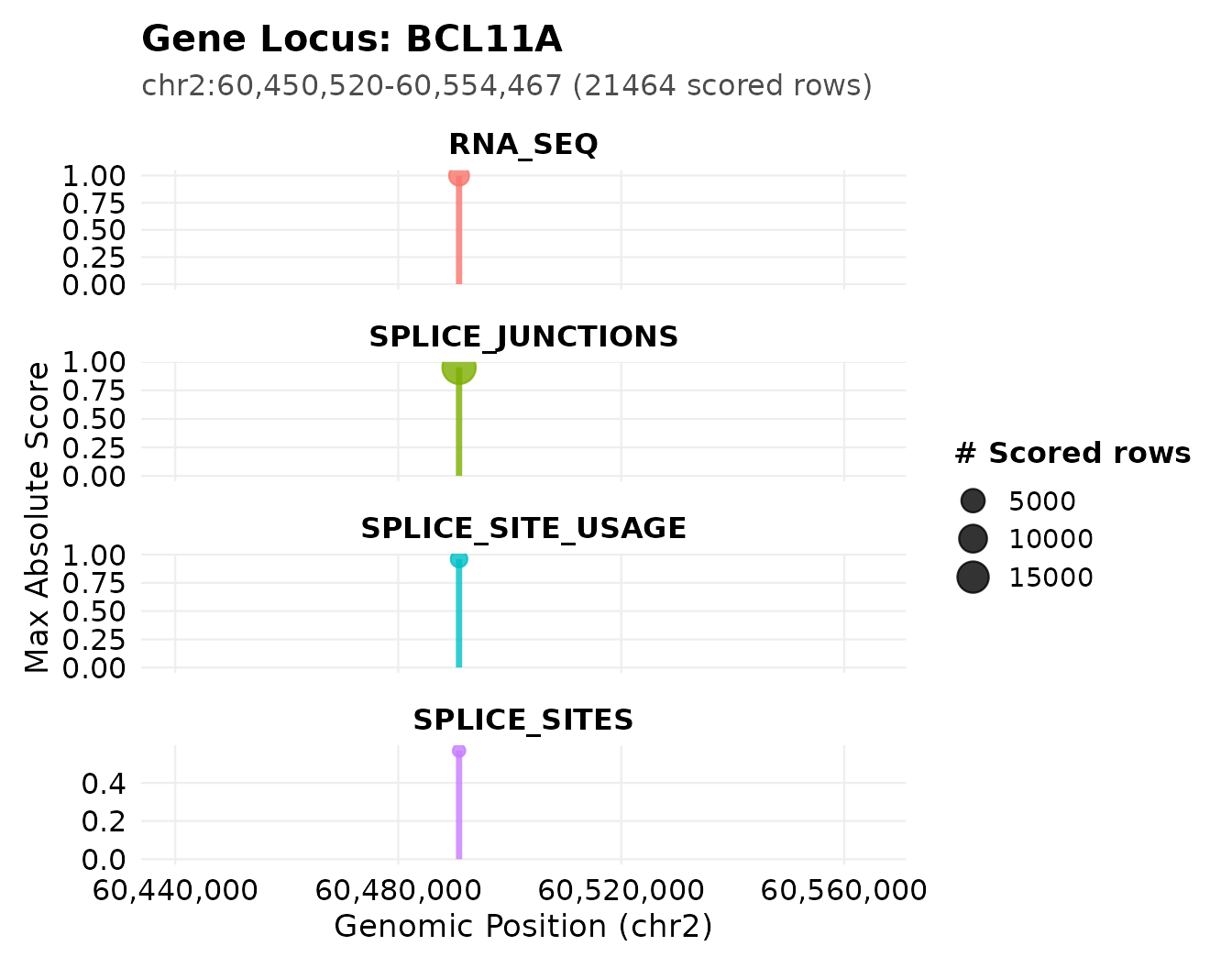

Scored rows across the BCL11A locus, split by modality. Only the modalities with rows annotated to BCL11A appear.

Reporting

av_create_report(obj) is zero-setup: the default spec (av_report_template_default()) carries auto_compute = TRUE, so statistics missing from $stats are computed before the block that needs them renders.

# open = FALSE keeps the vignette build from launching a browser. The report
# template loads DT, which is a Suggests dependency.
if (requireNamespace("DT", quietly = TRUE)) {
  report <- av_create_report(
    obj,
    output_file = file.path(tempdir(), "alphavar_report.html"),
    open        = FALSE
  )
  print(file.exists(report))
}
#> Rendering modular report to: /tmp/RtmpK2PIut/alphavar_report.html
#> [1] TRUE

Which blocks a report contains is set through its spec rather than through av_create_report(); the one content argument on the function is top_n_genes, which overrides the gene count in every gene_deep_dive block. Build a spec interactively in the Shiny Report tab, which provides block-by-block controls and YAML export, or programmatically with av_report_add_block() and av_report_remove_block(). A spec you build yourself computes nothing on its own unless you set auto_compute = TRUE on it, which guards against silently stale statistics.

PDF export additionally needs a Chrome or Chromium binary, which is why it is shown but not run:

av_export_pdf(obj, output_file = file.path(tempdir(), "alphavar_report.pdf"))

Interactive exploration

# Not evaluated here: both calls start a Shiny server and block the session.
av_run_shiny(obj)

av_explore(system.file("extdata", "bcl11a_rs1427407_scores.csv.gz", package = "AlphaVaR"))

The app exposes the pipeline in eight tabs:

Dashboard: counts, score distribution and saturation, directionality
Biological Landscape: region, TSS and custom annotation views
Causal Prioritization: the aggregation, specificity, target-mapping and ranking pipeline, split into a slow setup step and a fast re-ranking step
Single-Group Enrichment: ridges, volcano and enrichment bars with adjustable rarity and FDR thresholds
Group Comparison: pairwise, versus-reference and top-N intersection modes
Genomic View: locus and interval exploration
Data Explorer: searchable, filterable table
Report: assemble, preview and export a report spec

Summary

Import                    av_import_csv, av_set_active_score
   ↓
Overview                  av_overview_summary, av_plot_distribution
   ↓
Localization tests        av_calc_enrichment (Fisher)
                          av_calc_shift, av_compare_groups (rank-based)
   ↓
Specificity               av_calc_specificity (tau, per and across)
   ↓
Target and priority       av_map_targets, av_prioritize
   ↓
Output                    av_create_report, av_run_shiny

Every stage reads and returns an AlphaVarSet, and every filter or score switch clears the cached statistics, so plots and reports run after the calculation they depend on.

Session info

sessionInfo()
#> R version 4.6.1 (2026-06-24)
#> Platform: x86_64-pc-linux-gnu
#> Running under: Ubuntu 24.04.4 LTS
#> 
#> Matrix products: default
#> BLAS:   /usr/lib/x86_64-linux-gnu/openblas-pthread/libblas.so.3 
#> LAPACK: /usr/lib/x86_64-linux-gnu/openblas-pthread/libopenblasp-r0.3.26.so;  LAPACK version 3.12.0
#> 
#> locale:
#>  [1] LC_CTYPE=C.UTF-8       LC_NUMERIC=C           LC_TIME=C.UTF-8       
#>  [4] LC_COLLATE=C.UTF-8     LC_MONETARY=C.UTF-8    LC_MESSAGES=C.UTF-8   
#>  [7] LC_PAPER=C.UTF-8       LC_NAME=C              LC_ADDRESS=C          
#> [10] LC_TELEPHONE=C         LC_MEASUREMENT=C.UTF-8 LC_IDENTIFICATION=C   
#> 
#> time zone: UTC
#> tzcode source: system (glibc)
#> 
#> attached base packages:
#> [1] stats     graphics  grDevices utils     datasets  methods   base     
#> 
#> other attached packages:
#> [1] ggplot2_4.0.3  dplyr_1.2.1    AlphaVaR_1.0.0
#> 
#> loaded via a namespace (and not attached):
#>   [1] DBI_1.3.0                               
#>   [2] bitops_1.1-0                            
#>   [3] rlang_1.3.0                             
#>   [4] magrittr_2.0.5                          
#>   [5] otel_0.2.0                              
#>   [6] matrixStats_1.5.0                       
#>   [7] ggridges_0.5.7                          
#>   [8] compiler_4.6.1                          
#>   [9] RSQLite_3.53.3                          
#>  [10] GenomicFeatures_1.64.0                  
#>  [11] png_0.1-9                               
#>  [12] systemfonts_1.3.2                       
#>  [13] vctrs_0.7.3                             
#>  [14] stringr_1.6.0                           
#>  [15] pkgconfig_2.0.3                         
#>  [16] crayon_1.5.3                            
#>  [17] fastmap_1.2.0                           
#>  [18] XVector_0.52.0                          
#>  [19] labeling_0.4.3                          
#>  [20] utf8_1.2.6                              
#>  [21] Rsamtools_2.28.0                        
#>  [22] promises_1.5.0                          
#>  [23] rmarkdown_2.31                          
#>  [24] tzdb_0.5.0                              
#>  [25] UCSC.utils_1.8.0                        
#>  [26] ragg_1.5.2                              
#>  [27] purrr_1.2.2                             
#>  [28] bit_4.6.0                               
#>  [29] xfun_0.60                               
#>  [30] cachem_1.1.0                            
#>  [31] cigarillo_1.2.1                         
#>  [32] GenomeInfoDb_1.48.0                     
#>  [33] jsonlite_2.0.0                          
#>  [34] blob_1.3.0                              
#>  [35] later_1.4.8                             
#>  [36] DelayedArray_0.38.2                     
#>  [37] BiocParallel_1.46.0                     
#>  [38] parallel_4.6.1                          
#>  [39] R6_2.6.1                                
#>  [40] bslib_0.12.0                            
#>  [41] stringi_1.8.9                           
#>  [42] RColorBrewer_1.1-3                      
#>  [43] rtracklayer_1.72.0                      
#>  [44] GenomicRanges_1.64.0                    
#>  [45] jquerylib_0.1.4                         
#>  [46] Rcpp_1.1.2                              
#>  [47] Seqinfo_1.2.0                           
#>  [48] SummarizedExperiment_1.42.0             
#>  [49] knitr_1.51                              
#>  [50] readr_2.2.0                             
#>  [51] IRanges_2.46.0                          
#>  [52] httpuv_1.6.17                           
#>  [53] Matrix_1.7-5                            
#>  [54] tidyselect_1.2.1                        
#>  [55] abind_1.4-8                             
#>  [56] yaml_2.3.12                             
#>  [57] codetools_0.2-20                        
#>  [58] curl_7.1.0                              
#>  [59] lattice_0.22-9                          
#>  [60] tibble_3.3.1                            
#>  [61] Biobase_2.72.0                          
#>  [62] shiny_1.14.0                            
#>  [63] withr_3.0.3                             
#>  [64] KEGGREST_1.52.2                         
#>  [65] S7_0.2.2                                
#>  [66] evaluate_1.0.5                          
#>  [67] desc_1.4.3                              
#>  [68] Biostrings_2.80.1                       
#>  [69] pillar_1.11.1                           
#>  [70] MatrixGenerics_1.24.0                   
#>  [71] DT_0.34.0                               
#>  [72] stats4_4.6.1                            
#>  [73] shinyjs_2.1.1                           
#>  [74] generics_0.1.4                          
#>  [75] vroom_1.7.1                             
#>  [76] RCurl_1.98-1.19                         
#>  [77] S4Vectors_0.50.1                        
#>  [78] hms_1.1.4                               
#>  [79] scales_1.4.0                            
#>  [80] xtable_1.8-8                            
#>  [81] glue_1.8.1                              
#>  [82] tools_4.6.1                             
#>  [83] BiocIO_1.22.0                           
#>  [84] TxDb.Hsapiens.UCSC.hg38.knownGene_3.22.0
#>  [85] GenomicAlignments_1.48.0                
#>  [86] forcats_1.0.1                           
#>  [87] fs_2.1.0                                
#>  [88] XML_3.99-0.23                           
#>  [89] grid_4.6.1                              
#>  [90] tidyr_1.3.2                             
#>  [91] crosstalk_1.2.2                         
#>  [92] AnnotationDbi_1.74.0                    
#>  [93] restfulr_0.0.17                         
#>  [94] cli_3.6.6                               
#>  [95] textshaping_1.0.5                       
#>  [96] S4Arrays_1.12.0                         
#>  [97] viridisLite_0.4.3                       
#>  [98] gtable_0.3.6                            
#>  [99] sass_0.4.10                             
#> [100] digest_0.6.39                           
#> [101] BiocGenerics_0.58.1                     
#> [102] SparseArray_1.12.2                      
#> [103] ggrepel_0.9.8                           
#> [104] org.Hs.eg.db_3.23.1                     
#> [105] rjson_0.2.23                            
#> [106] htmlwidgets_1.6.4                       
#> [107] farver_2.1.2                            
#> [108] memoise_2.0.1                           
#> [109] htmltools_0.5.9                         
#> [110] pkgdown_2.2.1                           
#> [111] lifecycle_1.0.5                         
#> [112] httr_1.4.8                              
#> [113] mime_0.13                               
#> [114] bit64_4.8.2

Karim Marhaba

2026-08-14