Creates a publication-ready visualization of differential effects across
groups. Requires av_compare_groups() to have been run first.
Supports both 2-group and multi-group comparisons.
Usage
av_plot_comparison(
  obj,
  label_top_n = 10,
  style = c("effect_size", "boxplots", "ridges"),
  sig_threshold = 0.05,
  comparison_name = NULL
)
Arguments
- obj
An
AlphaVarSetobject with$stats$comparisonspopulated.- label_top_n
Integer. Number of top significant items to label (default 10).
- style
Character. One of "effect_size" (default, a lollipop forest of per-item median differences), "boxplots", or "ridges".
- sig_threshold
Numeric. P-adjusted threshold for significance (default 0.05).
- comparison_name
Character. Name of the comparison to plot. If NULL (default), uses the first available comparison.
Details
The plot shows score distributions side-by-side for the groups, highlighting items with the largest significant differences. Significance stars are added based on adjusted p-values:
*** : p_adj < 0.001
** : p_adj < 0.01
* : p_adj < 0.05
ns : not significant
Interpretation
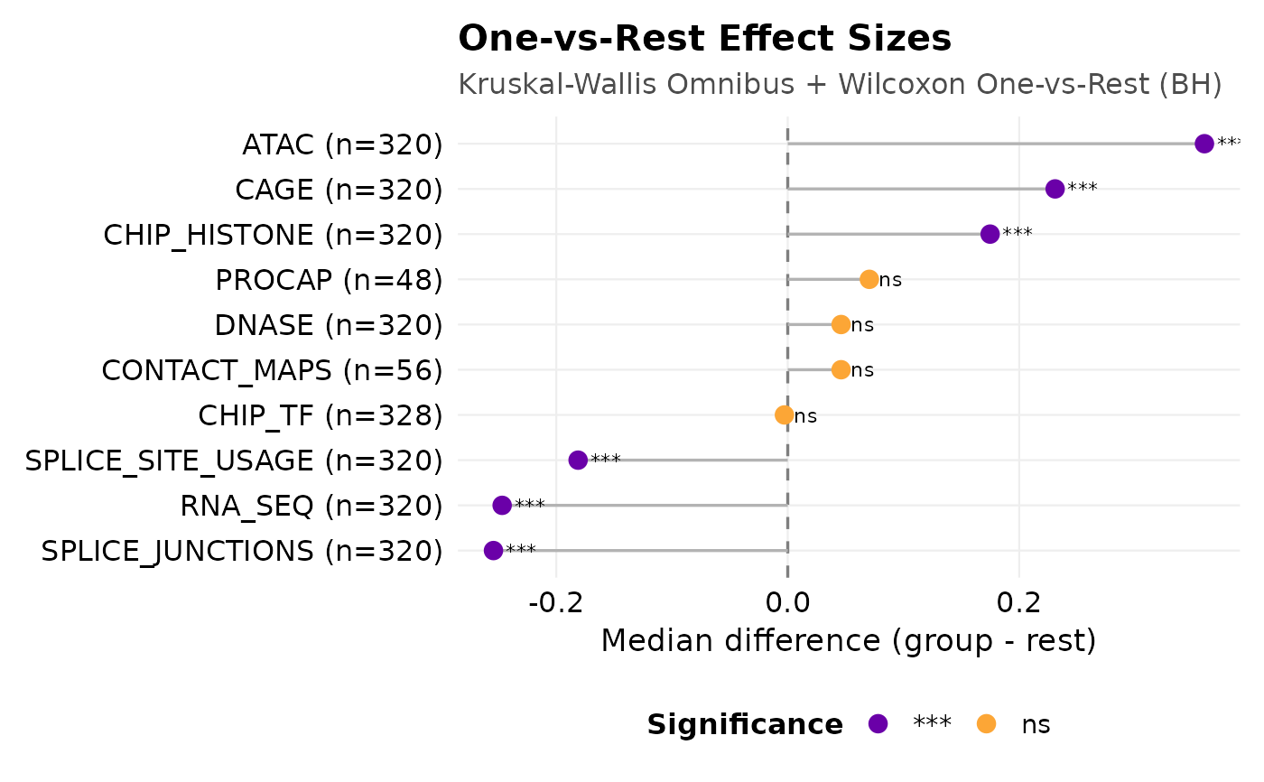
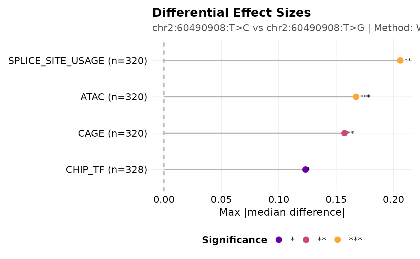
Items labeled with *** (p < 0.001) show the strongest differential effects between groups. A large median difference combined with high significance suggests biologically meaningful group-specific regulation. Items with 'ns' (not significant) show no evidence of differential effects at the given sample size.
Examples
example_file <- system.file("extdata", "bcl11a_rs1427407_example.csv", package = "AlphaVaR")
obj <- av_import_csv(example_file)
#> Reading bcl11a_rs1427407_example.csv ...
# Item-stratified: each output_type is tested for a T>C vs T>G allele difference.
obj <- av_compare_groups(obj, group_by = "variant_id", compare_by = "output_type")
#> Warning: 1 items skipped due to insufficient sample size (n < 5 ): SPLICE_SITES
head(obj$stats$comparisons[["variant_id_by_output_type"]]$results_tidy, 3)
#> # A tibble: 3 × 16
#> item group_1 group_2 n_1 n_2 median_1 median_2 median_diff p_val
#> <chr> <chr> <chr> <int> <int> <dbl> <dbl> <dbl> <dbl>
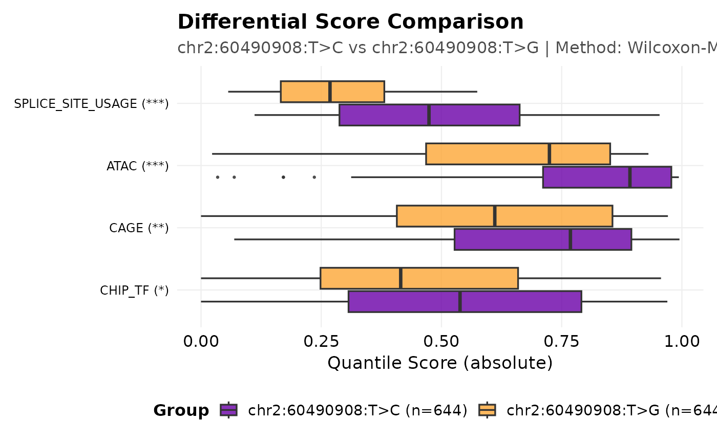
#> 1 SPLICE_SIT… chr2:6… chr2:6… 160 160 0.474 0.268 0.206 0
#> 2 ATAC chr2:6… chr2:6… 160 160 0.892 0.725 0.167 9.70e-13
#> 3 CAGE chr2:6… chr2:6… 160 160 0.768 0.611 0.157 3.94e- 4
#> # ℹ 7 more variables: effect_size <dbl>, effect_type <chr>, method <chr>,
#> # epsilon_sq <dbl>, kw_p <dbl>, p_adj <dbl>, significance_stars <chr>
av_plot_comparison(obj, label_top_n = 5)
 av_plot_comparison(obj, style = "boxplots", label_top_n = 4)
 # A one-vs-rest sweep carries no item column, so only the forest style applies.
obj <- av_calc_shift(obj, group_by = "output_type")
#> Warning: 1 element(s) dropped (n < 5 in one arm): SPLICE_SITES
av_plot_comparison(obj, comparison_name = "output_type_vs_rest")
# A one-vs-rest sweep carries no item column, so only the forest style applies.
obj <- av_calc_shift(obj, group_by = "output_type")
#> Warning: 1 element(s) dropped (n < 5 in one arm): SPLICE_SITES
av_plot_comparison(obj, comparison_name = "output_type_vs_rest")