Unified entry point for single-score distribution views over raw
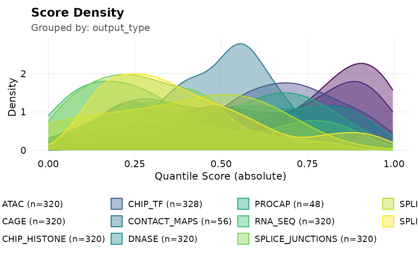
obj$data, stratified by group_by. style = "density"
overlays per-group densities; "ecdf" draws cumulative curves;
"directionality" shows the signed loss/gain balance; "ridges"
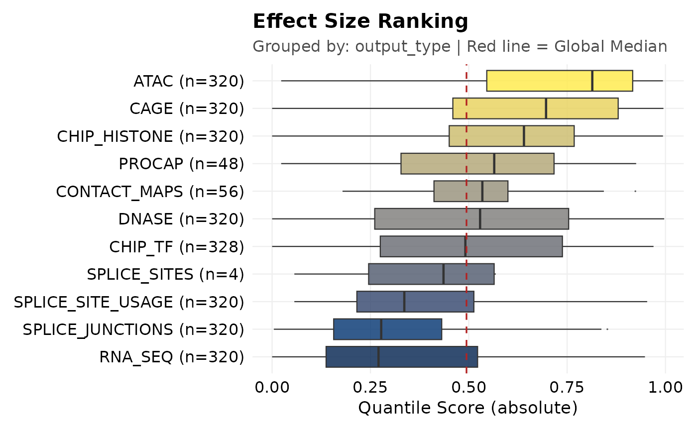
stacks per-group densities; "boxplots" ranks groups by median;
"calibration" plots raw against quantile score to expose saturation.
Usage
av_plot_distribution(
  obj,
  style = c("density", "ecdf", "directionality", "ridges", "boxplots", "calibration"),
  group_by = "output_type",
  abs_score = TRUE,
  filter_groups = NULL,
  drop_na = TRUE,
  orientation = c("horizontal", "vertical"),
  add_jitter = FALSE,
  loss_color = "#B22222",
  gain_color = "#2E8B57",
  outlier_handling = c("clip", "pseudolog"),
  clip_probs = c(0.005, 0.995),
  max_points = 10000L
)
Arguments
- obj
An
AlphaVarSetobject.- style
One of
"density","ecdf","directionality","ridges","boxplots","calibration".- group_by
Character. Column to stratify by (default
"output_type").- abs_score
Logical. Use absolute scores (default
TRUE). Ignored by"directionality"(which needs signed scores) and"calibration"(which plots both score columns directly).- filter_groups
Optional character vector of groups to keep.
- drop_na
Logical. Drop rows with NA group or score (default
TRUE).- orientation
"horizontal"(default) or"vertical", used by the"boxplots"style.- add_jitter
Logical. Overlay jittered points on
"boxplots"(defaultFALSE).- loss_color, gain_color
Colours for the
"directionality"diverging fill.- outlier_handling
For
"calibration":"clip"(default, zoom to theclip_probspercentile band and pin outliers to the margin) or"pseudolog"(signed pseudo-log10 raw axis).- clip_probs
Numeric length-2. Percentile bounds for
"clip"(defaultc(0.005, 0.995)).- max_points
Integer. For
"calibration", the maximum number of points to draw; larger inputs are down-sampled reproducibly (default10000).
Interpretation
Groups shifted to the right (or above the global-median line) carry systematically higher impact scores; broad shapes mean heterogeneous effects. In directionality, a skew towards negative values is repressive and positive is activating. In calibration, points stacked at the saturation band (|quantile| > 0.99) but spread horizontally mark variants where the raw score, not the quantile, carries the magnitude.
Examples
example_file <- system.file("extdata", "bcl11a_rs1427407_example.csv", package = "AlphaVaR")
obj <- av_import_csv(example_file)
#> Reading bcl11a_rs1427407_example.csv ...
av_plot_distribution(obj, style = "density")
 av_plot_distribution(obj, style = "boxplots", group_by = "output_type")