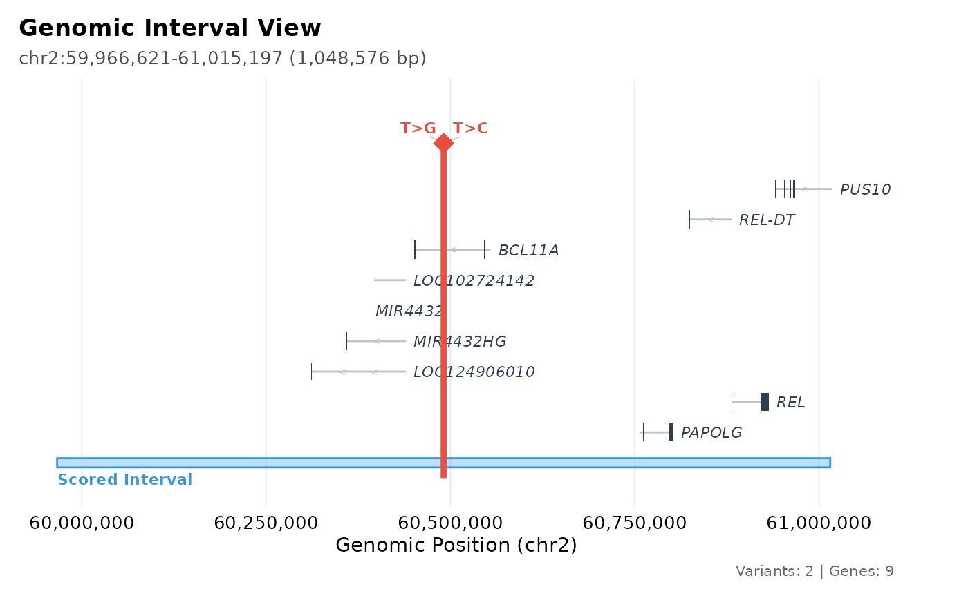
Creates a multi-track visualization of the scored genomic interval similar to the UCSC Genome Browser or AlphaGenome's native view. Shows the scored interval with gene transcripts and variant positions.
Usage
av_plot_interval(
  obj,
  txdb = NULL,
  show_all_transcripts = FALSE,
  variant_color = "#E74C3C",
  gene_colors = c(exon = "#2C3E50", intron = "#BDC3C7"),
  label_genes = TRUE,
  highlight_variant = NULL
)
Arguments
- obj
An
AlphaVarSetobject.- txdb
A TxDb object for transcript annotations (e.g., TxDb.Hsapiens.UCSC.hg38.knownGene). If NULL, only variant positions are shown without gene models.
- show_all_transcripts
Logical. If FALSE (default), show only the longest transcript per gene. If TRUE, show all transcripts.
- variant_color
Color for variant marker(s). Default "red".
- gene_colors
Named vector of colors for gene features. Recognized slots:
exon(rectangle fill, also used for gene labels) andintron(transcript line and strand-direction arrows). Defaults provided.- label_genes
Logical. Label gene names on the plot? Default TRUE.
- highlight_variant
Character. Specific variant_id to highlight (optional).
Details
The transcript models are a function of the TxDb and the plotted window only, so they are cached for the session: replotting the same interval after a filter or a score switch does not query the TxDb again.
Interpretation
This view provides genomic context for the scored region. Variant markers (red diamonds) show the exact positions of scored variants relative to gene structures (exons, introns, UTRs). Variants falling within exons may affect protein coding; variants in promoters or UTRs may affect gene regulation. Strand arrows indicate transcription direction.
Examples
example_file <- system.file("extdata", "bcl11a_rs1427407_example.csv",
package = "AlphaVaR")
obj <- av_import_csv(example_file)
#> Reading bcl11a_rs1427407_example.csv ...
# The window comes from scored_interval, the markers from variant_id.
unique(obj$data$scored_interval)
#> [1] "chr2:59966621-61015197:."
unique(obj$data$variant_id)
#> [1] "chr2:60490908:T>C" "chr2:60490908:T>G"
av_plot_interval(obj)
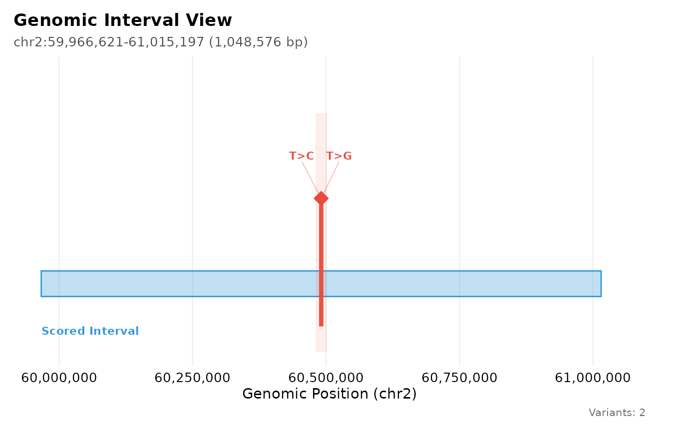
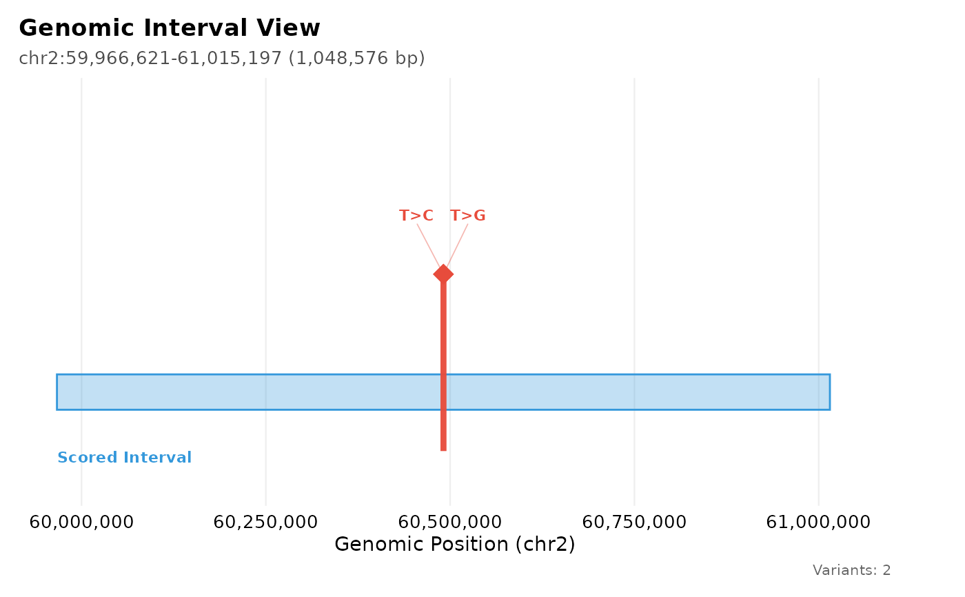 # Both alleles sit at chr2:60490908; highlight_variant shades one of them.
av_plot_interval(obj, highlight_variant = "chr2:60490908:T>C")
# Both alleles sit at chr2:60490908; highlight_variant shades one of them.
av_plot_interval(obj, highlight_variant = "chr2:60490908:T>C")
 # Gene models are optional: they need a TxDb, a ~1 GB Suggests package.
if (requireNamespace("TxDb.Hsapiens.UCSC.hg38.knownGene", quietly = TRUE)) {
print(av_plot_interval(
obj,
txdb = TxDb.Hsapiens.UCSC.hg38.knownGene::TxDb.Hsapiens.UCSC.hg38.knownGene,
show_all_transcripts = FALSE
))
}
#> Warning: Dropped 88 orphan transcript rows with no associated gene_id from the TxDb annotation.
#> 'select()' returned 1:1 mapping between keys and columns
# Gene models are optional: they need a TxDb, a ~1 GB Suggests package.
if (requireNamespace("TxDb.Hsapiens.UCSC.hg38.knownGene", quietly = TRUE)) {
print(av_plot_interval(
obj,
txdb = TxDb.Hsapiens.UCSC.hg38.knownGene::TxDb.Hsapiens.UCSC.hg38.knownGene,
show_all_transcripts = FALSE
))
}
#> Warning: Dropped 88 orphan transcript rows with no associated gene_id from the TxDb annotation.
#> 'select()' returned 1:1 mapping between keys and columns