Visualizes variants along genomic coordinates for a specific gene or region.
Uses the variant position from variant_id (format: chr:pos:ref>alt).
Arguments
- obj
An
AlphaVarSetobject.- gene_name
The gene to plot (filters variants for this gene).
- flank_bp
Number of base pairs to extend the plotting window when the TxDb lookup fails and only the variant range is available (default 0). The TxDb success path uses a 10% gene-span flank with a 1 kb minimum and ignores this argument.
- color_by
Column to map to color (default "output_type").
Interpretation
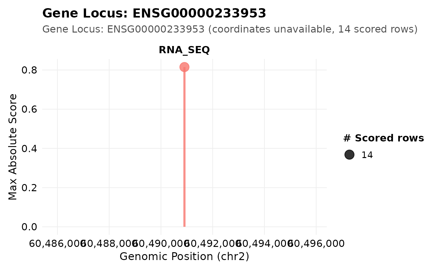
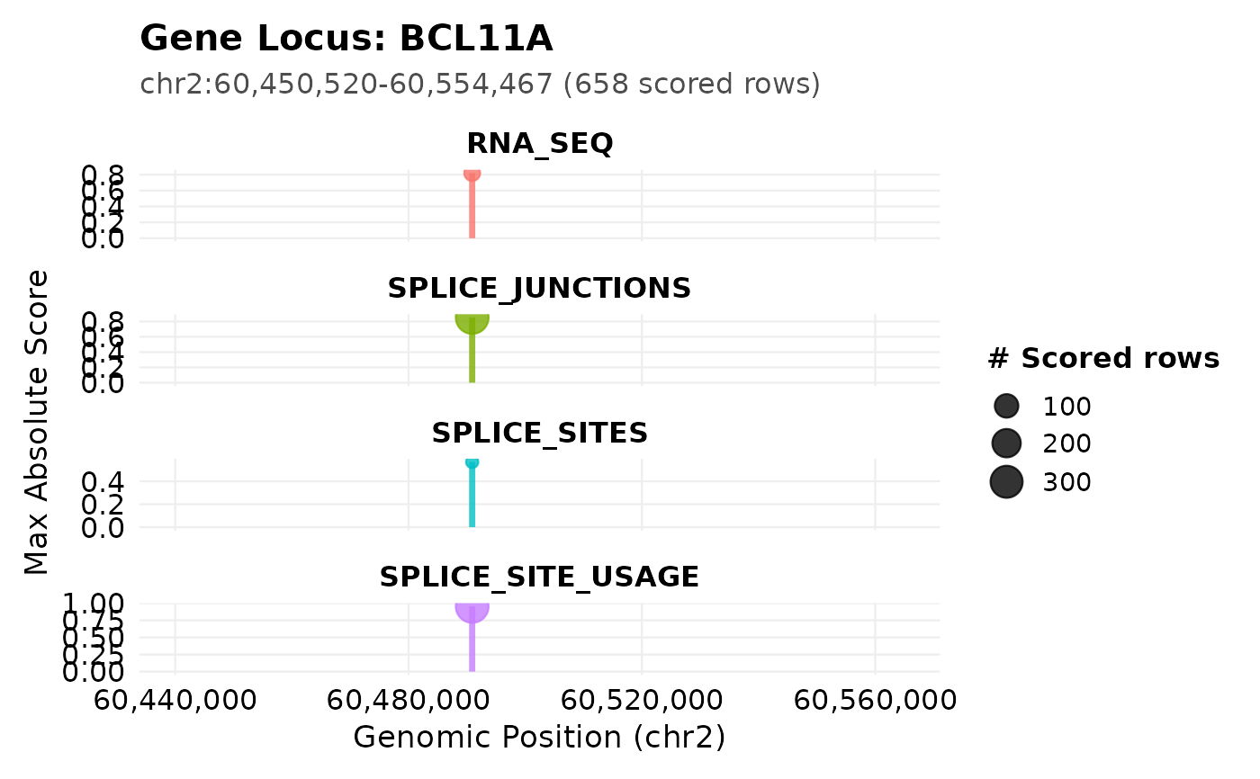
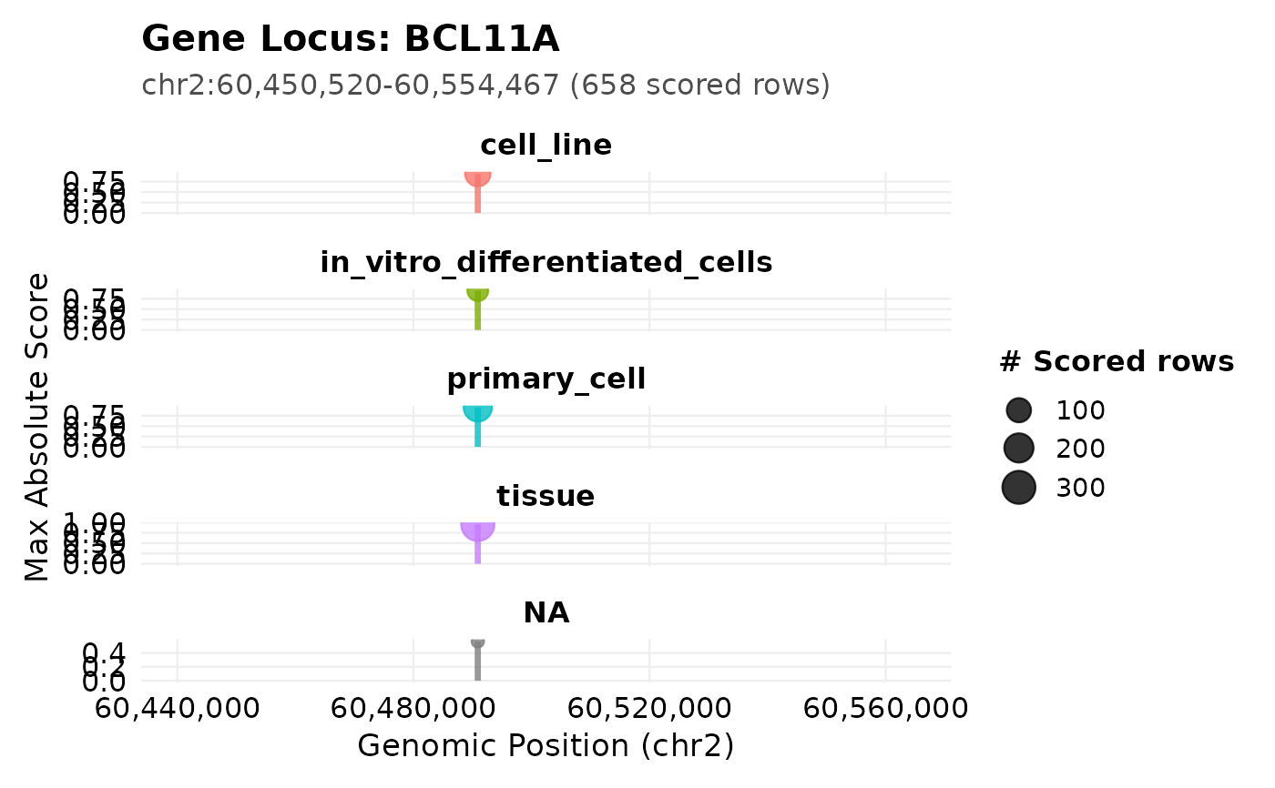
Tall lollipops indicate variants with high predicted impact at that genomic position. Clusters of high-scoring variants may indicate regulatory hotspots. Differences between facets (modalities) reveal tissue-specific effects at the same genomic position. Large points indicate multiple scored rows at that position.
Examples
example_file <- system.file("extdata", "bcl11a_rs1427407_example.csv",
package = "AlphaVaR")
obj <- av_import_csv(example_file)
#> Reading bcl11a_rs1427407_example.csv ...
# The filter runs on AlphaGenome's own gene_name column, so pick a symbol
# that the export actually carries.
head(sort(table(obj$data$gene_name), decreasing = TRUE), 3)
#>
#> BCL11A RNU1-32P MIR4432
#> 658 23 20
# Stem height is the maximum absolute value of the active score column.
obj$meta$active_score
#> [1] "quantile_score"
av_plot_locus(obj, gene_name = "BCL11A")
 # color_by both colours and facets, so a column with few elements stays legible.
av_plot_locus(obj, gene_name = "BCL11A", color_by = "biosample_type")
# color_by both colours and facets, so a column with few elements stays legible.
av_plot_locus(obj, gene_name = "BCL11A", color_by = "biosample_type")
 # flank_bp widens the window only when the TxDb symbol lookup fails, as it
# does for an unmapped Ensembl gene id: the plot then spans the variants alone.
av_plot_locus(obj, gene_name = "ENSG00000233953", flank_bp = 5000)
# flank_bp widens the window only when the TxDb symbol lookup fails, as it
# does for an unmapped Ensembl gene id: the plot then spans the variants alone.
av_plot_locus(obj, gene_name = "ENSG00000233953", flank_bp = 5000)