Plot Target vs Background Score Distribution

Plot showing variant scores from a target group versus the background (all other variants). Target membership is defined by either a logical column (e.g., is_HAR) or a value match on a categorical column (e.g., gene_name == "FOXP2"), the same logic as av_compare_target(). Reads the cached comparison from obj$stats$comparisons[[<key>]] and hard-errors if it is missing. Run av_compare_target() first.

Usage

av_plot_target(
  obj,
  target_col,
  target_value = TRUE,
  style = c("violin", "ecdf", "density"),
  abs_score = TRUE,
  show_pvalue = TRUE,
  target_color = "#E41A1C",
  bg_color = "#377EB8",
  labels = NULL
)

Arguments

obj

An AlphaVarSet with cached target comparison stats.

target_col

Character. Column name defining target membership.

target_value

Value to match against target_col. Default TRUE for logical columns; for character/factor columns supply the specific element (e.g., a gene symbol).

style

Character. One of "violin" (default), "ecdf", or "density".

abs_score

Logical. If TRUE (default), uses absolute scores.

show_pvalue

Logical. If TRUE (default), displays the cached p-value.

target_color

Color for the target group (default "#E41A1C").

bg_color

Color for the background (default "#377EB8").

labels

Optional named character vector to override the auto-derived group labels, e.g. c(target = "Inside ROI", background = "Outside"). When NULL (default), labels come from the column: logical columns give target_col / "Not target_col", categorical columns give target_value / "Background".

Value

A ggplot object.

Interpretation

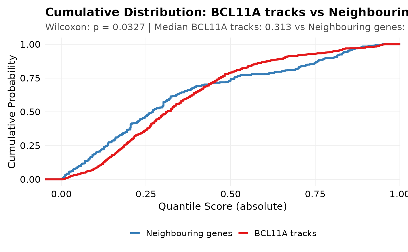
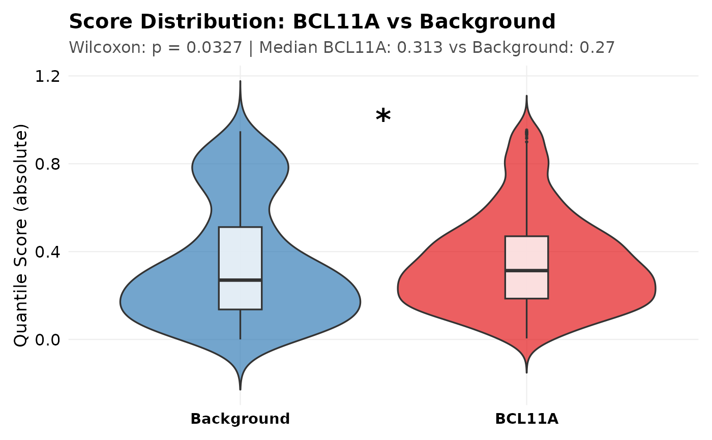
A significant p-value with a higher target median indicates the target group carries stronger predicted effects than background, supporting its functional relevance. The violin width and density shape reveal whether the signal comes from many moderate variants or a few extreme ones.

Examples

example_file <- system.file("extdata", "bcl11a_rs1427407_example.csv", package = "AlphaVaR")
obj <- av_import_csv(example_file)
#> Reading bcl11a_rs1427407_example.csv ...

# gene_name is categorical, so the target is one of its elements: tracks
# assigned to BCL11A itself against those of the neighbouring genes.
obj <- av_compare_target(obj, target_col = "gene_name", target_value = "BCL11A")
#> Warning: Dropped 1712 of 2676 rows with NA in 'gene_name', 'quantile_score'.
obj$stats$comparisons[["gene_name=BCL11A"]]$results_tidy
#> # A tibble: 1 × 12
#>   group  n_group n_rest median_group median_rest median_diff  p_val  p_adj
#>   <chr>    <int>  <int>        <dbl>       <dbl>       <dbl>  <dbl>  <dbl>
#> 1 BCL11A     658    306        0.313       0.270      0.0434 0.0327 0.0327
#> # ℹ 4 more variables: effect_size <dbl>, effect_type <chr>, method <chr>,
#> #   significance_stars <chr>

av_plot_target(obj, target_col = "gene_name", target_value = "BCL11A")
#> Warning: av_plot_target: dropped 1712 of 2676 rows with NA in 'gene_name' or 'quantile_score'.


av_plot_target(obj, target_col = "gene_name", target_value = "BCL11A",
               style = "ecdf",
               labels = c(target = "BCL11A tracks", background = "Neighbouring genes"))
#> Warning: av_plot_target: dropped 1712 of 2676 rows with NA in 'gene_name' or 'quantile_score'.